

Welcome to the final Computer Vision project in the Artificial Intelligence Nanodegree program!
In this project, you’ll combine your knowledge of computer vision techniques and deep learning to build and end-to-end facial keypoint recognition system! Facial keypoints include points around the eyes, nose, and mouth on any face and are used in many applications, from facial tracking to emotion recognition.
There are three main parts to this project:
Part 1 : Investigating OpenCV, pre-processing, and face detection
Part 2 : Training a Convolutional Neural Network (CNN) to detect facial keypoints
Part 3 : Putting parts 1 and 2 together to identify facial keypoints on any image!
*Here’s what you need to know to complete the project:
In this notebook, some template code has already been provided for you, and you will need to implement additional functionality to successfully complete this project. You will not need to modify the included code beyond what is requested.
a. Sections that begin with ‘(IMPLEMENTATION)’ in the header indicate that the following block of code will require additional functionality which you must provide. Instructions will be provided for each section, and the specifics of the implementation are marked in the code block with a ‘TODO’ statement. Please be sure to read the instructions carefully!
In addition to implementing code, there will be questions that you must answer which relate to the project and your implementation.
a. Each section where you will answer a question is preceded by a ‘Question X’ header.
b. Carefully read each question and provide thorough answers in the following text boxes that begin with ‘Answer:’.
Note: Code and Markdown cells can be executed using the Shift + Enter keyboard shortcut. Markdown cells can be edited by double-clicking the cell to enter edit mode.
The rubric contains optional suggestions for enhancing the project beyond the minimum requirements. If you decide to pursue the “(Optional)” sections, you should include the code in this IPython notebook.
Your project submission will be evaluated based on your answers to each of the questions and the code implementations you provide.
Each part of the notebook is further broken down into separate steps. Feel free to use the links below to navigate the notebook.
In this project you will get to explore a few of the many computer vision algorithms built into the OpenCV library. This expansive computer vision library is now almost 20 years old and still growing!
The project itself is broken down into three large parts, then even further into separate steps. Make sure to read through each step, and complete any sections that begin with ‘(IMPLEMENTATION)’ in the header; these implementation sections may contain multiple TODOs that will be marked in code. For convenience, we provide links to each of these steps below.
Part 1 : Investigating OpenCV, pre-processing, and face detection
Part 2 : Training a Convolutional Neural Network (CNN) to detect facial keypoints
Part 3 : Putting parts 1 and 2 together to identify facial keypoints on any image!
Have you ever wondered how Facebook automatically tags images with your friends’ faces? Or how high-end cameras automatically find and focus on a certain person’s face? Applications like these depend heavily on the machine learning task known as face detection - which is the task of automatically finding faces in images containing people.
At its root face detection is a classification problem - that is a problem of distinguishing between distinct classes of things. With face detection these distinct classes are 1) images of human faces and 2) everything else.
We use OpenCV’s implementation of Haar feature-based cascade classifiers to detect human faces in images. OpenCV provides many pre-trained face detectors, stored as XML files on github. We have downloaded one of these detectors and stored it in the detector_architectures directory.
In the next python cell, we load in the required libraries for this section of the project.
# Import required libraries for this section

%matplotlib inline

import numpy as np
import matplotlib.pyplot as plt
import math
import cv2                     # OpenCV library for computer vision
from PIL import Image
import time
Next, we load in and display a test image for performing face detection.
Note: by default OpenCV assumes the ordering of our image’s color channels are Blue, then Green, then Red. This is slightly out of order with most image types we’ll use in these experiments, whose color channels are ordered Red, then Green, then Blue. In order to switch the Blue and Red channels of our test image around we will use OpenCV’s cvtColor function, which you can read more about by checking out some of its documentation located here. This is a general utility function that can do other transformations too like converting a color image to grayscale, and transforming a standard color image to HSV color space.
# Load in color image for face detection
image = cv2.imread('images/test_image_1.jpg')

# Convert the image to RGB colorspace
image = cv2.cvtColor(image, cv2.COLOR_BGR2RGB)

# Plot our image using subplots to specify a size and title
fig = plt.figure(figsize = (8,8))
ax1 = fig.add_subplot(111)
ax1.set_xticks([])
ax1.set_yticks([])

ax1.set_title('Original Image')
ax1.imshow(image)
<matplotlib.image.AxesImage at 0x7fc46dff2160>

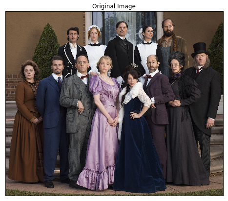
There are a lot of people - and faces - in this picture. 13 faces to be exact! In the next code cell, we demonstrate how to use a Haar Cascade classifier to detect all the faces in this test image.
This face detector uses information about patterns of intensity in an image to reliably detect faces under varying light conditions. So, to use this face detector, we’ll first convert the image from color to grayscale.
Then, we load in the fully trained architecture of the face detector – found in the file haarcascade_frontalface_default.xml - and use it on our image to find faces!
To learn more about the parameters of the detector see this post.
# Convert the RGB  image to grayscale
gray = cv2.cvtColor(image, cv2.COLOR_RGB2GRAY)

# Extract the pre-trained face detector from an xml file
face_cascade = cv2.CascadeClassifier('detector_architectures/haarcascade_frontalface_default.xml')

# Detect the faces in image
faces = face_cascade.detectMultiScale(gray, 4, 6)

# Print the number of faces detected in the image
print('Number of faces detected:', len(faces))

# Make a copy of the orginal image to draw face detections on
image_with_detections = np.copy(image)

# Get the bounding box for each detected face
for (x,y,w,h) in faces:
    # Add a red bounding box to the detections image
    cv2.rectangle(image_with_detections, (x,y), (x+w,y+h), (255,0,0), 3)


# Display the image with the detections
fig = plt.figure(figsize = (8,8))
ax1 = fig.add_subplot(111)
ax1.set_xticks([])
ax1.set_yticks([])

ax1.set_title('Image with Face Detections')
ax1.imshow(image_with_detections)
Number of faces detected: 13


<matplotlib.image.AxesImage at 0x7fc46d6fe0f0>

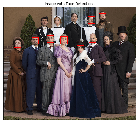
In the above code, faces is a numpy array of detected faces, where each row corresponds to a detected face. Each detected face is a 1D array with four entries that specifies the bounding box of the detected face. The first two entries in the array (extracted in the above code as x and y) specify the horizontal and vertical positions of the top left corner of the bounding box. The last two entries in the array (extracted here as w and h) specify the width and height of the box.
There are other pre-trained detectors available that use a Haar Cascade Classifier - including full human body detectors, license plate detectors, and more. A full list of the pre-trained architectures can be found here.
To test your eye detector, we’ll first read in a new test image with just a single face.
# Load in color image for face detection
image = cv2.imread('images/james.jpg')

# Convert the image to RGB colorspace
image = cv2.cvtColor(image, cv2.COLOR_BGR2RGB)

# Plot the RGB image
fig = plt.figure(figsize = (6,6))
ax1 = fig.add_subplot(111)
ax1.set_xticks([])
ax1.set_yticks([])

ax1.set_title('Original Image')
ax1.imshow(image)
<matplotlib.image.AxesImage at 0x7fc4644454e0>

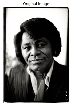
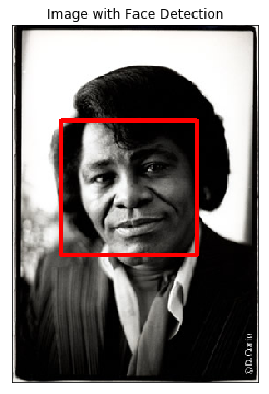
Notice that even though the image is a black and white image, we have read it in as a color image and so it will still need to be converted to grayscale in order to perform the most accurate face detection.
So, the next steps will be to convert this image to grayscale, then load OpenCV’s face detector and run it with parameters that detect this face accurately.
# Convert the RGB  image to grayscale
gray = cv2.cvtColor(image, cv2.COLOR_RGB2GRAY)

# Extract the pre-trained face detector from an xml file
face_cascade = cv2.CascadeClassifier('detector_architectures/haarcascade_frontalface_default.xml')

# Detect the faces in image
faces = face_cascade.detectMultiScale(gray, 1.25, 6)

# Print the number of faces detected in the image
print('Number of faces detected:', len(faces))

# Make a copy of the orginal image to draw face detections on
image_with_detections = np.copy(image)

# Get the bounding box for each detected face
for (x,y,w,h) in faces:
    # Add a red bounding box to the detections image
    cv2.rectangle(image_with_detections, (x,y), (x+w,y+h), (255,0,0), 3)


# Display the image with the detections
fig = plt.figure(figsize = (6,6))
ax1 = fig.add_subplot(111)
ax1.set_xticks([])
ax1.set_yticks([])

ax1.set_title('Image with Face Detection')
ax1.imshow(image_with_detections)
Number of faces detected: 1


<matplotlib.image.AxesImage at 0x7fc46439cf60>

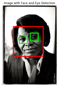
A Haar-cascade eye detector can be included in the same way that the face detector was and, in this first task, it will be your job to do just this.
To set up an eye detector, use the stored parameters of the eye cascade detector, called haarcascade_eye.xml, located in the detector_architectures subdirectory. In the next code cell, create your eye detector and store its detections.
A few notes before you get started:
First, make sure to give your loaded eye detector the variable name
eye_cascade
and give the list of eye regions you detect the variable name
eyes
Second, since we’ve already run the face detector over this image, you should only search for eyes within the rectangular face regions detected in faces. This will minimize false detections.
Lastly, once you’ve run your eye detector over the facial detection region, you should display the RGB image with both the face detection boxes (in red) and your eye detections (in green) to verify that everything works as expected.
# Make a copy of the original image to plot rectangle detections
image_with_detections = np.copy(image)

# Loop over the detections and draw their corresponding face detection boxes
for (x,y,w,h) in faces:
    cv2.rectangle(image_with_detections, (x,y), (x+w,y+h),(255,0,0), 3)

# Do not change the code above this comment!


## TODO: Add eye detection, using haarcascade_eye.xml, to the current face detector algorithm
eye_cascade = cv2.CascadeClassifier('detector_architectures/haarcascade_eye.xml')
eyes = eye_cascade.detectMultiScale(image_with_detections, 2, 1)
## TODO: Loop over the eye detections and draw their corresponding boxes in green on image_with_detections
for (x,y,w,h) in eyes:
    # Add a red bounding box to the detections image
    cv2.rectangle(image_with_detections, (x,y), (x+w,y+h), (0,255,0), 3)

# Plot the image with both faces and eyes detected
fig = plt.figure(figsize = (6,6))
ax1 = fig.add_subplot(111)
ax1.set_xticks([])
ax1.set_yticks([])

ax1.set_title('Image with Face and Eye Detection')
ax1.imshow(image_with_detections)
<matplotlib.image.AxesImage at 0x7fc4643800f0>

It’s time to kick it up a notch, and add face and eye detection to your laptop’s camera! Afterwards, you’ll be able to show off your creation like in the gif shown below - made with a completed version of the code!
<img src=”images/laptop_face_detector_example.gif” width=400 height=300/>
Notice that not all of the detections here are perfect - and your result need not be perfect either. You should spend a small amount of time tuning the parameters of your detectors to get reasonable results, but don’t hold out for perfection. If we wanted perfection we’d need to spend a ton of time tuning the parameters of each detector, cleaning up the input image frames, etc. You can think of this as more of a rapid prototype.
The next cell contains code for a wrapper function called laptop_camera_face_eye_detector that, when called, will activate your laptop’s camera. You will place the relevant face and eye detection code in this wrapper function to implement face/eye detection and mark those detections on each image frame that your camera captures.
Before adding anything to the function, you can run it to get an idea of how it works - a small window should pop up showing you the live feed from your camera; you can press any key to close this window.
Note: Mac users may find that activating this function kills the kernel of their notebook every once in a while. If this happens to you, just restart your notebook’s kernel, activate cell(s) containing any crucial import statements, and you’ll be good to go!
### Add face and eye detection to this laptop camera function
# Make sure to draw out all faces/eyes found in each frame on the shown video feed

import cv2
import time

# wrapper function for face/eye detection with your laptop camera
def laptop_camera_go():
    # Create instance of video capturer
    cv2.namedWindow("face detection activated")
    vc =cv2.VideoCapture(0)

    # Try to get the first frame
    if vc.isOpened():
        rval, frame = vc.read()
    else:
        rval = False

    # Keep the video stream open
    while rval:
        # Plot the image from camera with all the face and eye detections marked
        cv2.imshow("face detection activated", frame)

        # Exit functionality - press any key to exit laptop video
        key = cv2.waitKey(20)
        if key > 0: # Exit by pressing any key
            # Destroy windows
            cv2.destroyAllWindows()

            # Make sure window closes on OSx
            for i in range (1,5):
                cv2.waitKey(1)
            return

        # Read next frame
        time.sleep(0.05)             # control framerate for computation - default 20 frames per sec
        rval, frame = vc.read()
# Call the laptop camera face/eye detector function above
laptop_camera_go()
Image quality is an important aspect of any computer vision task. Typically, when creating a set of images to train a deep learning network, significant care is taken to ensure that training images are free of visual noise or artifacts that hinder object detection. While computer vision algorithms - like a face detector - are typically trained on ‘nice’ data such as this, new test data doesn’t always look so nice!
When applying a trained computer vision algorithm to a new piece of test data one often cleans it up first before feeding it in. This sort of cleaning - referred to as pre-processing - can include a number of cleaning phases like blurring, de-noising, color transformations, etc., and many of these tasks can be accomplished using OpenCV.
In this short subsection we explore OpenCV’s noise-removal functionality to see how we can clean up a noisy image, which we then feed into our trained face detector.
In the next cell, we create an artificial noisy version of the previous multi-face image. This is a little exaggerated - we don’t typically get images that are this noisy - but image noise, or ‘grainy-ness’ in a digitial image - is a fairly common phenomenon.
# Load in the multi-face test image again
image = cv2.imread('images/test_image_1.jpg')

# Convert the image copy to RGB colorspace
image = cv2.cvtColor(image, cv2.COLOR_BGR2RGB)

# Make an array copy of this image
image_with_noise = np.asarray(image)

# Create noise - here we add noise sampled randomly from a Gaussian distribution: a common model for noise
noise_level = 40
noise = np.random.randn(image.shape[0],image.shape[1],image.shape[2])*noise_level

# Add this noise to the array image copy
image_with_noise = image_with_noise + noise

# Convert back to uint8 format
image_with_noise = np.asarray([np.uint8(np.clip(i,0,255)) for i in image_with_noise])

# Plot our noisy image!
fig = plt.figure(figsize = (8,8))
ax1 = fig.add_subplot(111)
ax1.set_xticks([])
ax1.set_yticks([])

ax1.set_title('Noisy Image')
ax1.imshow(image_with_noise)
<matplotlib.image.AxesImage at 0x7fc4640d94a8>

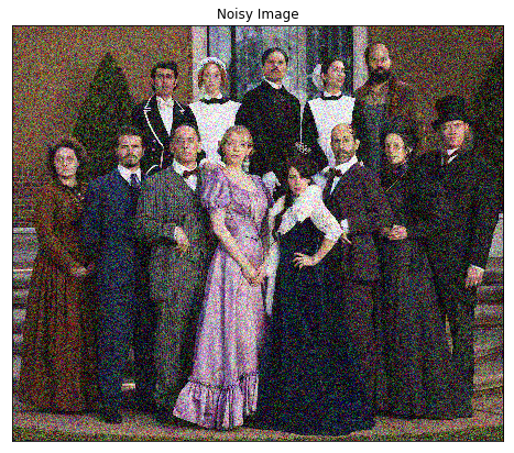
In the context of face detection, the problem with an image like this is that - due to noise - we may miss some faces or get false detections.
In the next cell we apply the same trained OpenCV detector with the same settings as before, to see what sort of detections we get.
# Convert the RGB  image to grayscale
gray_noise = cv2.cvtColor(image_with_noise, cv2.COLOR_RGB2GRAY)

# Extract the pre-trained face detector from an xml file
face_cascade = cv2.CascadeClassifier('detector_architectures/haarcascade_frontalface_default.xml')

# Detect the faces in image
faces = face_cascade.detectMultiScale(gray_noise, 4, 6)

# Print the number of faces detected in the image
print('Number of faces detected:', len(faces))

# Make a copy of the orginal image to draw face detections on
image_with_detections = np.copy(image_with_noise)

# Get the bounding box for each detected face
for (x,y,w,h) in faces:
    # Add a red bounding box to the detections image
    cv2.rectangle(image_with_detections, (x,y), (x+w,y+h), (255,0,0), 3)


# Display the image with the detections
fig = plt.figure(figsize = (8,8))
ax1 = fig.add_subplot(111)
ax1.set_xticks([])
ax1.set_yticks([])

ax1.set_title('Noisy Image with Face Detections')
ax1.imshow(image_with_detections)
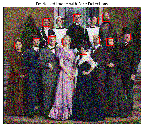
Number of faces detected: 12


<matplotlib.image.AxesImage at 0x7fc4640b4668>


With this added noise we now miss one of the faces!
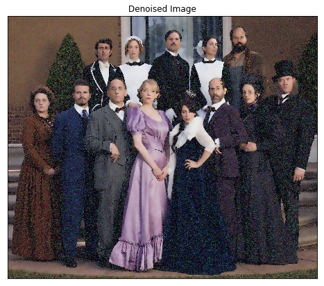
Time to get your hands dirty: using OpenCV’s built in color image de-noising functionality called fastNlMeansDenoisingColored - de-noise this image enough so that all the faces in the image are properly detected. Once you have cleaned the image in the next cell, use the cell that follows to run our trained face detector over the cleaned image to check out its detections.
You can find its [official documentation here](documentation for denoising and a useful example here.
Note: you can keep all parameters except photo_render fixed as shown in the second link above. Play around with the value of this parameter - see how it affects the resulting cleaned image.
## TODO: Use OpenCV's built in color image de-noising function to clean up our noisy image!


denoised_image = cv2.fastNlMeansDenoisingColored(image_with_noise,None,20,20,7,21)
#denoised_image = cv2.fastNlMeansDenoisingColored(image_with_noise, None, 13, 13, 7, 21)
# your final de-noised image (should be RGB)
# Plot our denoised image
fig = plt.figure(figsize = (8,8))
ax1 = fig.add_subplot(111)
ax1.set_xticks([])
ax1.set_yticks([])
ax1.set_title('Denoised Image')
ax1.imshow(denoised_image)
<matplotlib.image.AxesImage at 0x7fc46408bcc0>

## TODO: Run the face detector on the de-noised image to improve your detections and display the result
gray_noise = cv2.cvtColor(denoised_image, cv2.COLOR_RGB2GRAY)

# Extract the pre-trained face detector from an xml file
face_cascade = cv2.CascadeClassifier('detector_architectures/haarcascade_frontalface_default.xml')

# Detect the faces in image
faces = face_cascade.detectMultiScale(gray_noise, 4, 6)

# Print the number of faces detected in the image
print('Number of faces detected:', len(faces))

# Make a copy of the orginal image to draw face detections on
image_with_detections = np.copy(image_with_noise)

# Get the bounding box for each detected face
for (x,y,w,h) in faces:
    # Add a red bounding box to the detections image
    cv2.rectangle(image_with_detections, (x,y), (x+w,y+h), (255,0,0), 3)

fig = plt.figure(figsize = (8,8))
ax1 = fig.add_subplot(111)
ax1.set_xticks([])
ax1.set_yticks([])

ax1.set_title('De-Noised Image with Face Detections')
ax1.imshow(image_with_detections)
Number of faces detected: 13


<matplotlib.image.AxesImage at 0x7fc45c3ba6d8>

Now that we have developed a simple pipeline for detecting faces using OpenCV - let’s start playing around with a few fun things we can do with all those detected faces!
Edge detection is a concept that pops up almost everywhere in computer vision applications, as edge-based features (as well as features built on top of edges) are often some of the best features for e.g., object detection and recognition problems.
Edge detection is a dimension reduction technique - by keeping only the edges of an image we get to throw away a lot of non-discriminating information. And typically the most useful kind of edge-detection is one that preserves only the important, global structures (ignoring local structures that aren’t very discriminative). So removing local structures / retaining global structures is a crucial pre-processing step to performing edge detection in an image, and blurring can do just that.
Below is an animated gif showing the result of an edge-detected cat taken from Wikipedia, where the image is gradually blurred more and more prior to edge detection. When the animation begins you can’t quite make out what it’s a picture of, but as the animation evolves and local structures are removed via blurring the cat becomes visible in the edge-detected image.
<img src=”images/Edge_Image.gif” width=400 height=300/>
Edge detection is a convolution performed on the image itself, and you can read about Canny edge detection on this OpenCV documentation page.
In the cell below we load in a test image, then apply Canny edge detection on it. The original image is shown on the left panel of the figure, while the edge-detected version of the image is shown on the right. Notice how the result looks very busy - there are too many little details preserved in the image before it is sent to the edge detector. When applied in computer vision applications, edge detection should preserve global structure; doing away with local structures that don’t help describe what objects are in the image.
# Load in the image
image = cv2.imread('images/fawzia.jpg')

# Convert to RGB colorspace
image = cv2.cvtColor(image, cv2.COLOR_BGR2RGB)

# Convert to grayscale
gray = cv2.cvtColor(image, cv2.COLOR_RGB2GRAY)

# Perform Canny edge detection
edges = cv2.Canny(gray,100,200)

# Dilate the image to amplify edges
edges = cv2.dilate(edges, None)

# Plot the RGB and edge-detected image
fig = plt.figure(figsize = (15,15))
ax1 = fig.add_subplot(121)
ax1.set_xticks([])
ax1.set_yticks([])

ax1.set_title('Original Image')
ax1.imshow(image)

ax2 = fig.add_subplot(122)
ax2.set_xticks([])
ax2.set_yticks([])

ax2.set_title('Canny Edges')
ax2.imshow(edges, cmap='gray')
<matplotlib.image.AxesImage at 0x7fc45c3d7208>

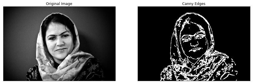
Without first blurring the image, and removing small, local structures, a lot of irrelevant edge content gets picked up and amplified by the detector (as shown in the right panel above).
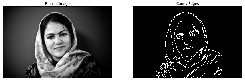
In the next cell, you will repeat this experiment - blurring the image first to remove these local structures, so that only the important boudnary details remain in the edge-detected image.
Blur the image by using OpenCV’s filter2d functionality - which is discussed in this documentation page - and use an averaging kernel of width equal to 4.
### TODO: Blur the test imageusing OpenCV's filter2d functionality,
# Use an averaging kernel, and a kernel width equal to 4

kernel = np.ones((4,4),np.float32)/16
blurred_image = cv2.filter2D(image, -1, kernel)

# Convert to RGB colorspace
image = cv2.cvtColor(blurred_image, cv2.COLOR_BGR2RGB)

# Convert to grayscale
gray = cv2.cvtColor(image, cv2.COLOR_RGB2GRAY)

# Perform Canny edge detection
edges = cv2.Canny(gray,100,200)

# Dilate the image to amplify edges
edges = cv2.dilate(edges, None)

## TODO: Then perform Canny edge detection and display the output
fig = plt.figure(figsize = (15,15))
ax1 = fig.add_subplot(121)
ax1.set_xticks([])
ax1.set_yticks([])

ax1.set_title('Blurred Image')
ax1.imshow(blurred_image)

ax2 = fig.add_subplot(122)
ax2.set_xticks([])
ax2.set_yticks([])

ax2.set_title('Canny Edges')
ax2.imshow(edges, cmap='gray')
<matplotlib.image.AxesImage at 0x7fc45c2ffd30>

If you film something like a documentary or reality TV, you must get permission from every individual shown on film before you can show their face, otherwise you need to blur it out - by blurring the face a lot (so much so that even the global structures are obscured)! This is also true for projects like Google’s StreetView maps - an enormous collection of mapping images taken from a fleet of Google vehicles. Because it would be impossible for Google to get the permission of every single person accidentally captured in one of these images they blur out everyone’s faces, the detected images must automatically blur the identity of detected people. Here’s a few examples of folks caught in the camera of a Google street view vehicle.
<img src=”images/streetview_example_1.jpg” width=400 height=300/> <img src=”images/streetview_example_2.jpg” width=400 height=300/>
Let’s try this out for ourselves. Use the face detection pipeline built above and what you know about using the filter2D to blur and image, and use these in tandem to hide the identity of the person in the following image - loaded in and printed in the next cell.
# Load in the image
image = cv2.imread('images/gus.jpg')

# Convert the image to RGB colorspace
image = cv2.cvtColor(image, cv2.COLOR_BGR2RGB)

# Display the image
fig = plt.figure(figsize = (6,6))
ax1 = fig.add_subplot(111)
ax1.set_xticks([])
ax1.set_yticks([])
ax1.set_title('Original Image')
ax1.imshow(image)
<matplotlib.image.AxesImage at 0x7fc45c1f2cf8>

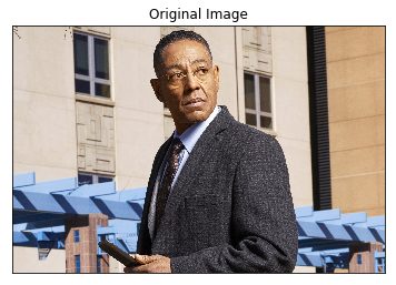
The idea here is to 1) automatically detect the face in this image, and then 2) blur it out! Make sure to adjust the parameters of the averaging blur filter to completely obscure this person’s identity.
## TODO: Implement face detection
# Convert the RGB  image to grayscale
gray_noise = cv2.cvtColor(image, cv2.COLOR_RGB2GRAY)

# Extract the pre-trained face detector from an xml file
face_cascade = cv2.CascadeClassifier('detector_architectures/haarcascade_frontalface_default.xml')

# Detect the faces in image
faces = face_cascade.detectMultiScale(gray_noise, 2, 2)

# Print the number of faces detected in the image
print('Number of faces detected:', len(faces))

# Make a copy of the orginal image to draw face detections on
image_with_detections = np.copy(image)

## TODO: Blur the bounding box around each detected face using an averaging filter and display the result
# Get the bounding box for each detected face
for (x,y,w,h) in faces:
    # Add a red bounding box to the detections image
    crop_img = image[y:y+h, x:x+w]
    crop_blurred_img = cv2.blur(crop_img, (50,50))
    image_with_detections[y:y+h, x:x+w] = crop_blurred_img


# Display the image with the detections
fig = plt.figure(figsize = (8,8))
ax1 = fig.add_subplot(111)
ax1.set_xticks([])
ax1.set_yticks([])

ax1.set_title('Face Detections')
ax1.imshow(image_with_detections)
Number of faces detected: 1


<matplotlib.image.AxesImage at 0x7fc45c1cd908>


In this optional task you can add identity protection to your laptop camera, using the previously completed code where you added face detection to your laptop camera - and the task above. You should be able to get reasonable results with little parameter tuning - like the one shown in the gif below.
<img src=”images/laptop_blurer_example.gif” width=400 height=300/>
As with the previous video task, to make this perfect would require significant effort - so don’t strive for perfection here, strive for reasonable quality.
The next cell contains code a wrapper function called laptop_camera_identity_hider that - when called - will activate your laptop’s camera. You need to place the relevant face detection and blurring code developed above in this function in order to blur faces entering your laptop camera’s field of view.
Before adding anything to the function you can call it to get a hang of how it works - a small window will pop up showing you the live feed from your camera, you can press any key to close this window.
Note: Mac users may find that activating this function kills the kernel of their notebook every once in a while. If this happens to you, just restart your notebook’s kernel, activate cell(s) containing any crucial import statements, and you’ll be good to go!
### Insert face detection and blurring code into the wrapper below to create an identity protector on your laptop!
import cv2
import time

def laptop_camera_go():
    # Create instance of video capturer
    cv2.namedWindow("face detection activated")
    vc = cv2.VideoCapture(0)

    # Try to get the first frame
    if vc.isOpened():
        rval, frame = vc.read()
    else:
        rval = False

    # Keep video stream open
    while rval:
        # Plot image from camera with detections marked
        cv2.imshow("face detection activated", frame)

        # Exit functionality - press any key to exit laptop video
        key = cv2.waitKey(20)
        if key > 0: # Exit by pressing any key
            # Destroy windows
            cv2.destroyAllWindows()

            for i in range (1,5):
                cv2.waitKey(1)
            return

        # Read next frame
        time.sleep(0.05)             # control framerate for computation - default 20 frames per sec
        rval, frame = vc.read()
# Run laptop identity hider
laptop_camera_go()
OpenCV is often used in practice with other machine learning and deep learning libraries to produce interesting results. In this stage of the project you will create your own end-to-end pipeline - employing convolutional networks in keras along with OpenCV - to apply a “selfie” filter to streaming video and images.
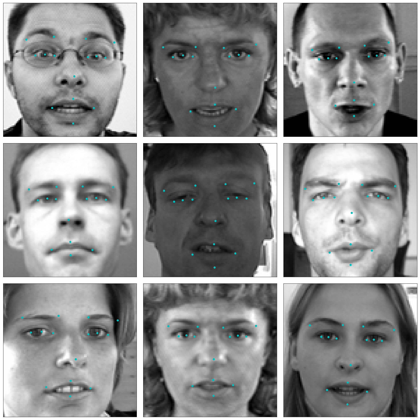
You will start by creating and then training a convolutional network that can detect facial keypoints in a small dataset of cropped images of human faces. We then guide you towards OpenCV to expanding your detection algorithm to more general images. What are facial keypoints? Let’s take a look at some examples.
<img src=”images/keypoints_test_results.png” width=400 height=300/>
Facial keypoints (also called facial landmarks) are the small blue-green dots shown on each of the faces in the image above - there are 15 keypoints marked in each image. They mark important areas of the face - the eyes, corners of the mouth, the nose, etc. Facial keypoints can be used in a variety of machine learning applications from face and emotion recognition to commercial applications like the image filters popularized by Snapchat.
Below we illustrate a filter that, using the results of this section, automatically places sunglasses on people in images (using the facial keypoints to place the glasses correctly on each face). Here, the facial keypoints have been colored lime green for visualization purposes.
<img src=”images/obamas_with_shades.png” width=1000 height=1000/>
But first things first: how can we make a facial keypoint detector? Well, at a high level, notice that facial keypoint detection is a regression problem. A single face corresponds to a set of 15 facial keypoints (a set of 15 corresponding $(x, y)$ coordinates, i.e., an output point). Because our input data are images, we can employ a convolutional neural network to recognize patterns in our images and learn how to identify these keypoint given sets of labeled data.
In order to train a regressor, we need a training set - a set of facial image / facial keypoint pairs to train on. For this we will be using this dataset from Kaggle. We’ve already downloaded this data and placed it in the data directory. Make sure that you have both the training and test data files. The training dataset contains several thousand $96 \times 96$ grayscale images of cropped human faces, along with each face’s 15 corresponding facial keypoints (also called landmarks) that have been placed by hand, and recorded in $(x, y)$ coordinates. This wonderful resource also has a substantial testing set, which we will use in tinkering with our convolutional network.
To load in this data, run the Python cell below - notice we will load in both the training and testing sets.
The load_data function is in the included utils.py file.
from utils import *

# Load training set
X_train, y_train = load_data()
print("X_train.shape == {}".format(X_train.shape))
print("y_train.shape == {}; y_train.min == {:.3f}; y_train.max == {:.3f}".format(
    y_train.shape, y_train.min(), y_train.max()))

# Load testing set
X_test, _ = load_data(test=True)
print("X_test.shape == {}".format(X_test.shape))
Using TensorFlow backend.


X_train.shape == (2140, 96, 96, 1)
y_train.shape == (2140, 30); y_train.min == -0.920; y_train.max == 0.996
X_test.shape == (1783, 96, 96, 1)
The load_data function in utils.py originates from this excellent blog post, which you are strongly encouraged to read. Please take the time now to review this function. Note how the output values - that is, the coordinates of each set of facial landmarks - have been normalized to take on values in the range $[-1, 1]$, while the pixel values of each input point (a facial image) have been normalized to the range $[0,1]$.
Note: the original Kaggle dataset contains some images with several missing keypoints. For simplicity, the load_data function removes those images with missing labels from the dataset. As an optional extension, you are welcome to amend the load_data function to include the incomplete data points.
Execute the code cell below to visualize a subset of the training data.
import matplotlib.pyplot as plt
%matplotlib inline

fig = plt.figure(figsize=(20,20))
fig.subplots_adjust(left=0, right=1, bottom=0, top=1, hspace=0.05, wspace=0.05)
for i in range(9):
    ax = fig.add_subplot(3, 3, i + 1, xticks=[], yticks=[])
    plot_data(X_train[i], y_train[i], ax)

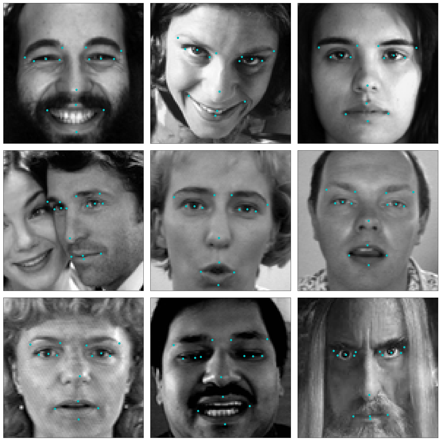
For each training image, there are two landmarks per eyebrow (four total), three per eye (six total), four for the mouth, and one for the tip of the nose.
Review the plot_data function in utils.py to understand how the 30-dimensional training labels in y_train are mapped to facial locations, as this function will prove useful for your pipeline.
In this section, you will specify a neural network for predicting the locations of facial keypoints. Use the code cell below to specify the architecture of your neural network. We have imported some layers that you may find useful for this task, but if you need to use more Keras layers, feel free to import them in the cell.
Your network should accept a $96 \times 96$ grayscale image as input, and it should output a vector with 30 entries, corresponding to the predicted (horizontal and vertical) locations of 15 facial keypoints. If you are not sure where to start, you can find some useful starting architectures in this blog, but you are not permitted to copy any of the architectures that you find online.
# Import deep learning resources from Keras
from keras.models import Sequential
from keras.layers import Convolution2D, MaxPooling2D, Dropout
from keras.layers import Flatten, Dense

## TODO: Specify a CNN architecture
# Your model should accept 96x96 pixel graysale images in
# It should have a fully-connected output layer with 30 values (2 for each facial keypoint)

model = Sequential()
model.add(Convolution2D(8, (3,3), input_shape=(96,96,1)))#X_train.shape[1:]))
model.add(MaxPooling2D(pool_size=(2, 2)))
# model.add(Dropout(0.3))

model.add(Convolution2D(16, (2,2), activation='relu'))
model.add(MaxPooling2D(pool_size=(2, 2)))
# model.add(Dropout(0.3))

model.add(Convolution2D(32, (2,2), activation='relu'))
model.add(MaxPooling2D(pool_size=(2, 2)))
# model.add(Dropout(0.3))

model.add(Flatten())
model.add(Dense(500))
model.add(Dropout(0.5))

model.add(Dense(30))

# Summarize the model
model.summary()
_________________________________________________________________
Layer (type)                 Output Shape              Param #
=================================================================
conv2d_1 (Conv2D)            (None, 94, 94, 8)         80
_________________________________________________________________
max_pooling2d_1 (MaxPooling2 (None, 47, 47, 8)         0
_________________________________________________________________
conv2d_2 (Conv2D)            (None, 46, 46, 16)        528
_________________________________________________________________
max_pooling2d_2 (MaxPooling2 (None, 23, 23, 16)        0
_________________________________________________________________
conv2d_3 (Conv2D)            (None, 22, 22, 32)        2080
_________________________________________________________________
max_pooling2d_3 (MaxPooling2 (None, 11, 11, 32)        0
_________________________________________________________________
flatten_1 (Flatten)          (None, 3872)              0
_________________________________________________________________
dense_1 (Dense)              (None, 500)               1936500
_________________________________________________________________
dropout_1 (Dropout)          (None, 500)               0
_________________________________________________________________
dense_2 (Dense)              (None, 30)                15030
=================================================================
Total params: 1,954,218
Trainable params: 1,954,218
Non-trainable params: 0
_________________________________________________________________
After specifying your architecture, you’ll need to compile and train the model to detect facial keypoints’
Use the compile method to configure the learning process. Experiment with your choice of optimizer; you may have some ideas about which will work best (SGD vs. RMSprop, etc), but take the time to empirically verify your theories.
Use the fit method to train the model. Break off a validation set by setting validation_split=0.2. Save the returned History object in the history variable.
Experiment with your model to minimize the validation loss (measured as mean squared error). A very good model will achieve about 0.0015 loss (though it’s possible to do even better). When you have finished training, save your model as an HDF5 file with file path my_model.h5.
from keras.optimizers import SGD, RMSprop, Adagrad, Adadelta, Adam, Adamax, Nadam

## TODO: Compile the model
history={}
epochs = 20
optimizers= ['SGD', 'RMSprop', 'Adagrad', 'Adadelta', 'Adam', 'Adamax', 'Nadam']
names= ['SGD', 'RMSprop', 'Adagrad', 'Adadelta', 'Adam', 'Adamax', 'Nadam']
for optimizer,name in zip(optimizers, names):
    model.compile(optimizer=optimizer, loss='mean_squared_error', metrics=['mse','accuracy'])
    ## TODO: Train the model
    print("evaliting optimizer " + name)
    history[name] = model.fit(X_train, y_train,
          validation_split=0.2,
          epochs=epochs, batch_size=10, verbose=1)
    ## TODO: Save the model as model.h5
    model.save('my_model_'+name+'.h5')
evaliting optimizer SGD
Train on 1712 samples, validate on 428 samples
Epoch 1/20
1712/1712 [==============================] - 2s 1ms/step - loss: 0.0473 - mean_squared_error: 0.0473 - acc: 0.3370 - val_loss: 0.0086 - val_mean_squared_error: 0.0086 - val_acc: 0.6822
Epoch 2/20
1712/1712 [==============================] - 1s 668us/step - loss: 0.0203 - mean_squared_error: 0.0203 - acc: 0.4019 - val_loss: 0.0072 - val_mean_squared_error: 0.0072 - val_acc: 0.6916
Epoch 3/20
1712/1712 [==============================] - 1s 716us/step - loss: 0.0168 - mean_squared_error: 0.0168 - acc: 0.4311 - val_loss: 0.0062 - val_mean_squared_error: 0.0062 - val_acc: 0.6939
Epoch 4/20
1712/1712 [==============================] - 1s 683us/step - loss: 0.0147 - mean_squared_error: 0.0147 - acc: 0.4702 - val_loss: 0.0058 - val_mean_squared_error: 0.0058 - val_acc: 0.6963
Epoch 5/20
1712/1712 [==============================] - 1s 668us/step - loss: 0.0136 - mean_squared_error: 0.0136 - acc: 0.4614 - val_loss: 0.0056 - val_mean_squared_error: 0.0056 - val_acc: 0.6939
Epoch 6/20
1712/1712 [==============================] - 1s 677us/step - loss: 0.0128 - mean_squared_error: 0.0128 - acc: 0.4871 - val_loss: 0.0056 - val_mean_squared_error: 0.0056 - val_acc: 0.6939
Epoch 7/20
1712/1712 [==============================] - 1s 674us/step - loss: 0.0122 - mean_squared_error: 0.0122 - acc: 0.5064 - val_loss: 0.0053 - val_mean_squared_error: 0.0053 - val_acc: 0.6939
Epoch 8/20
1712/1712 [==============================] - 1s 680us/step - loss: 0.0118 - mean_squared_error: 0.0118 - acc: 0.4901 - val_loss: 0.0051 - val_mean_squared_error: 0.0051 - val_acc: 0.6963
Epoch 9/20
1712/1712 [==============================] - 1s 672us/step - loss: 0.0113 - mean_squared_error: 0.0113 - acc: 0.5175 - val_loss: 0.0052 - val_mean_squared_error: 0.0052 - val_acc: 0.6939
Epoch 10/20
1712/1712 [==============================] - 1s 680us/step - loss: 0.0110 - mean_squared_error: 0.0110 - acc: 0.5129 - val_loss: 0.0052 - val_mean_squared_error: 0.0052 - val_acc: 0.6939
Epoch 11/20
1712/1712 [==============================] - 1s 682us/step - loss: 0.0109 - mean_squared_error: 0.0109 - acc: 0.5304 - val_loss: 0.0050 - val_mean_squared_error: 0.0050 - val_acc: 0.6963
Epoch 12/20
1712/1712 [==============================] - 1s 675us/step - loss: 0.0106 - mean_squared_error: 0.0106 - acc: 0.5275 - val_loss: 0.0048 - val_mean_squared_error: 0.0048 - val_acc: 0.6963
Epoch 13/20
1712/1712 [==============================] - 1s 672us/step - loss: 0.0104 - mean_squared_error: 0.0104 - acc: 0.5129 - val_loss: 0.0050 - val_mean_squared_error: 0.0050 - val_acc: 0.6963
Epoch 14/20
1712/1712 [==============================] - 1s 675us/step - loss: 0.0102 - mean_squared_error: 0.0102 - acc: 0.5210 - val_loss: 0.0050 - val_mean_squared_error: 0.0050 - val_acc: 0.6963
Epoch 15/20
1712/1712 [==============================] - 1s 678us/step - loss: 0.0100 - mean_squared_error: 0.0100 - acc: 0.5199 - val_loss: 0.0050 - val_mean_squared_error: 0.0050 - val_acc: 0.6963
Epoch 16/20
1712/1712 [==============================] - 1s 676us/step - loss: 0.0098 - mean_squared_error: 0.0098 - acc: 0.5660 - val_loss: 0.0047 - val_mean_squared_error: 0.0047 - val_acc: 0.6963
Epoch 17/20
1712/1712 [==============================] - 1s 686us/step - loss: 0.0096 - mean_squared_error: 0.0096 - acc: 0.5199 - val_loss: 0.0054 - val_mean_squared_error: 0.0054 - val_acc: 0.6963
Epoch 18/20
1712/1712 [==============================] - 1s 679us/step - loss: 0.0096 - mean_squared_error: 0.0096 - acc: 0.5567 - val_loss: 0.0050 - val_mean_squared_error: 0.0050 - val_acc: 0.6963
Epoch 19/20
1712/1712 [==============================] - 1s 686us/step - loss: 0.0095 - mean_squared_error: 0.0095 - acc: 0.5491 - val_loss: 0.0049 - val_mean_squared_error: 0.0049 - val_acc: 0.6963
Epoch 20/20
1712/1712 [==============================] - 1s 680us/step - loss: 0.0093 - mean_squared_error: 0.0093 - acc: 0.5514 - val_loss: 0.0049 - val_mean_squared_error: 0.0049 - val_acc: 0.6963
evaliting optimizer RMSprop
Train on 1712 samples, validate on 428 samples
Epoch 1/20
1712/1712 [==============================] - 2s 912us/step - loss: 0.0134 - mean_squared_error: 0.0134 - acc: 0.5800 - val_loss: 0.0050 - val_mean_squared_error: 0.0050 - val_acc: 0.7313
Epoch 2/20
1712/1712 [==============================] - 1s 825us/step - loss: 0.0053 - mean_squared_error: 0.0053 - acc: 0.6793 - val_loss: 0.0032 - val_mean_squared_error: 0.0032 - val_acc: 0.7079
Epoch 3/20
1712/1712 [==============================] - 1s 818us/step - loss: 0.0034 - mean_squared_error: 0.0034 - acc: 0.7027 - val_loss: 0.0027 - val_mean_squared_error: 0.0027 - val_acc: 0.7150
Epoch 4/20
1712/1712 [==============================] - 1s 821us/step - loss: 0.0029 - mean_squared_error: 0.0029 - acc: 0.7103 - val_loss: 0.0026 - val_mean_squared_error: 0.0026 - val_acc: 0.6752
Epoch 5/20
1712/1712 [==============================] - 1s 816us/step - loss: 0.0026 - mean_squared_error: 0.0026 - acc: 0.7272 - val_loss: 0.0027 - val_mean_squared_error: 0.0027 - val_acc: 0.7383
Epoch 6/20
1712/1712 [==============================] - 1s 821us/step - loss: 0.0023 - mean_squared_error: 0.0023 - acc: 0.7459 - val_loss: 0.0019 - val_mean_squared_error: 0.0019 - val_acc: 0.7266
Epoch 7/20
1712/1712 [==============================] - 1s 820us/step - loss: 0.0022 - mean_squared_error: 0.0022 - acc: 0.7418 - val_loss: 0.0029 - val_mean_squared_error: 0.0029 - val_acc: 0.7430
Epoch 8/20
1712/1712 [==============================] - 1s 819us/step - loss: 0.0020 - mean_squared_error: 0.0020 - acc: 0.7541 - val_loss: 0.0026 - val_mean_squared_error: 0.0026 - val_acc: 0.7313
Epoch 9/20
1712/1712 [==============================] - 1s 819us/step - loss: 0.0019 - mean_squared_error: 0.0019 - acc: 0.7611 - val_loss: 0.0021 - val_mean_squared_error: 0.0021 - val_acc: 0.7453
Epoch 10/20
1712/1712 [==============================] - 1s 824us/step - loss: 0.0017 - mean_squared_error: 0.0017 - acc: 0.7541 - val_loss: 0.0020 - val_mean_squared_error: 0.0020 - val_acc: 0.7430
Epoch 11/20
1712/1712 [==============================] - 1s 821us/step - loss: 0.0017 - mean_squared_error: 0.0017 - acc: 0.7745 - val_loss: 0.0032 - val_mean_squared_error: 0.0032 - val_acc: 0.7640
Epoch 12/20
1712/1712 [==============================] - 1s 829us/step - loss: 0.0016 - mean_squared_error: 0.0016 - acc: 0.7722 - val_loss: 0.0022 - val_mean_squared_error: 0.0022 - val_acc: 0.7383
Epoch 13/20
1712/1712 [==============================] - 1s 831us/step - loss: 0.0015 - mean_squared_error: 0.0015 - acc: 0.7751 - val_loss: 0.0022 - val_mean_squared_error: 0.0022 - val_acc: 0.7313
Epoch 14/20
1712/1712 [==============================] - 1s 826us/step - loss: 0.0014 - mean_squared_error: 0.0014 - acc: 0.7821 - val_loss: 0.0020 - val_mean_squared_error: 0.0020 - val_acc: 0.7430
Epoch 15/20
1712/1712 [==============================] - 1s 827us/step - loss: 0.0014 - mean_squared_error: 0.0014 - acc: 0.7985 - val_loss: 0.0021 - val_mean_squared_error: 0.0021 - val_acc: 0.7617
Epoch 16/20
1712/1712 [==============================] - 1s 826us/step - loss: 0.0013 - mean_squared_error: 0.0013 - acc: 0.7921 - val_loss: 0.0019 - val_mean_squared_error: 0.0019 - val_acc: 0.7360
Epoch 17/20
1712/1712 [==============================] - 1s 824us/step - loss: 0.0012 - mean_squared_error: 0.0012 - acc: 0.8014 - val_loss: 0.0023 - val_mean_squared_error: 0.0023 - val_acc: 0.7383
Epoch 18/20
1712/1712 [==============================] - 1s 823us/step - loss: 0.0012 - mean_squared_error: 0.0012 - acc: 0.7845 - val_loss: 0.0023 - val_mean_squared_error: 0.0023 - val_acc: 0.7313
Epoch 19/20
1712/1712 [==============================] - 1s 828us/step - loss: 0.0011 - mean_squared_error: 0.0011 - acc: 0.7961 - val_loss: 0.0016 - val_mean_squared_error: 0.0016 - val_acc: 0.7477
Epoch 20/20
1712/1712 [==============================] - 1s 826us/step - loss: 0.0011 - mean_squared_error: 0.0011 - acc: 0.8166 - val_loss: 0.0017 - val_mean_squared_error: 0.0017 - val_acc: 0.7710
evaliting optimizer Adagrad
Train on 1712 samples, validate on 428 samples
Epoch 1/20
1712/1712 [==============================] - 1s 850us/step - loss: 0.0110 - mean_squared_error: 0.0110 - acc: 0.7167 - val_loss: 0.0029 - val_mean_squared_error: 0.0029 - val_acc: 0.7523
Epoch 2/20
1712/1712 [==============================] - 1s 806us/step - loss: 0.0016 - mean_squared_error: 0.0016 - acc: 0.7582 - val_loss: 0.0018 - val_mean_squared_error: 0.0018 - val_acc: 0.7407
Epoch 3/20
1712/1712 [==============================] - 1s 796us/step - loss: 0.0013 - mean_squared_error: 0.0013 - acc: 0.7909 - val_loss: 0.0017 - val_mean_squared_error: 0.0017 - val_acc: 0.7617
Epoch 4/20
1712/1712 [==============================] - 1s 821us/step - loss: 0.0012 - mean_squared_error: 0.0012 - acc: 0.7874 - val_loss: 0.0017 - val_mean_squared_error: 0.0017 - val_acc: 0.7710
Epoch 5/20
1712/1712 [==============================] - 1s 838us/step - loss: 0.0011 - mean_squared_error: 0.0011 - acc: 0.7938 - val_loss: 0.0017 - val_mean_squared_error: 0.0017 - val_acc: 0.7593
Epoch 6/20
1712/1712 [==============================] - 1s 808us/step - loss: 0.0010 - mean_squared_error: 0.0010 - acc: 0.7897 - val_loss: 0.0016 - val_mean_squared_error: 0.0016 - val_acc: 0.7850
Epoch 7/20
1712/1712 [==============================] - 1s 812us/step - loss: 9.4005e-04 - mean_squared_error: 9.4005e-04 - acc: 0.8084 - val_loss: 0.0016 - val_mean_squared_error: 0.0016 - val_acc: 0.7897
Epoch 8/20
1712/1712 [==============================] - 1s 799us/step - loss: 8.8547e-04 - mean_squared_error: 8.8547e-04 - acc: 0.8055 - val_loss: 0.0016 - val_mean_squared_error: 0.0016 - val_acc: 0.7734
Epoch 9/20
1712/1712 [==============================] - 1s 799us/step - loss: 8.4998e-04 - mean_squared_error: 8.4998e-04 - acc: 0.8119 - val_loss: 0.0017 - val_mean_squared_error: 0.0017 - val_acc: 0.7804
Epoch 10/20
1712/1712 [==============================] - 1s 803us/step - loss: 8.1516e-04 - mean_squared_error: 8.1516e-04 - acc: 0.8265 - val_loss: 0.0016 - val_mean_squared_error: 0.0016 - val_acc: 0.7827
Epoch 11/20
1712/1712 [==============================] - 1s 801us/step - loss: 7.9446e-04 - mean_squared_error: 7.9446e-04 - acc: 0.8236 - val_loss: 0.0016 - val_mean_squared_error: 0.0016 - val_acc: 0.7734
Epoch 12/20
1712/1712 [==============================] - 1s 824us/step - loss: 7.5944e-04 - mean_squared_error: 7.5944e-04 - acc: 0.8067 - val_loss: 0.0016 - val_mean_squared_error: 0.0016 - val_acc: 0.7687
Epoch 13/20
1712/1712 [==============================] - 1s 795us/step - loss: 7.4420e-04 - mean_squared_error: 7.4420e-04 - acc: 0.8277 - val_loss: 0.0016 - val_mean_squared_error: 0.0016 - val_acc: 0.7897
Epoch 14/20
1712/1712 [==============================] - 1s 801us/step - loss: 7.1811e-04 - mean_squared_error: 7.1811e-04 - acc: 0.8265 - val_loss: 0.0016 - val_mean_squared_error: 0.0016 - val_acc: 0.7780
Epoch 15/20
1712/1712 [==============================] - 1s 796us/step - loss: 7.0079e-04 - mean_squared_error: 7.0079e-04 - acc: 0.8300 - val_loss: 0.0015 - val_mean_squared_error: 0.0015 - val_acc: 0.7874
Epoch 16/20
1712/1712 [==============================] - 1s 795us/step - loss: 6.8631e-04 - mean_squared_error: 6.8631e-04 - acc: 0.8353 - val_loss: 0.0015 - val_mean_squared_error: 0.0015 - val_acc: 0.7734
Epoch 17/20
1712/1712 [==============================] - 1s 813us/step - loss: 6.5833e-04 - mean_squared_error: 6.5833e-04 - acc: 0.8300 - val_loss: 0.0015 - val_mean_squared_error: 0.0015 - val_acc: 0.7921
Epoch 18/20
1712/1712 [==============================] - 1s 800us/step - loss: 6.5497e-04 - mean_squared_error: 6.5497e-04 - acc: 0.8359 - val_loss: 0.0016 - val_mean_squared_error: 0.0016 - val_acc: 0.7827
Epoch 19/20
1712/1712 [==============================] - 1s 805us/step - loss: 6.5164e-04 - mean_squared_error: 6.5164e-04 - acc: 0.8329 - val_loss: 0.0016 - val_mean_squared_error: 0.0016 - val_acc: 0.7757
Epoch 20/20
1712/1712 [==============================] - 1s 797us/step - loss: 6.3056e-04 - mean_squared_error: 6.3056e-04 - acc: 0.8411 - val_loss: 0.0016 - val_mean_squared_error: 0.0016 - val_acc: 0.7827
evaliting optimizer Adadelta
Train on 1712 samples, validate on 428 samples
Epoch 1/20
1712/1712 [==============================] - 2s 1ms/step - loss: 6.5545e-04 - mean_squared_error: 6.5545e-04 - acc: 0.8417 - val_loss: 0.0017 - val_mean_squared_error: 0.0017 - val_acc: 0.7687
Epoch 2/20
1712/1712 [==============================] - 2s 1ms/step - loss: 6.2871e-04 - mean_squared_error: 6.2871e-04 - acc: 0.8364 - val_loss: 0.0015 - val_mean_squared_error: 0.0015 - val_acc: 0.7850
Epoch 3/20
1712/1712 [==============================] - 2s 1ms/step - loss: 6.1787e-04 - mean_squared_error: 6.1787e-04 - acc: 0.8376 - val_loss: 0.0016 - val_mean_squared_error: 0.0016 - val_acc: 0.7710
Epoch 4/20
1712/1712 [==============================] - 2s 1ms/step - loss: 6.2465e-04 - mean_squared_error: 6.2465e-04 - acc: 0.8446 - val_loss: 0.0015 - val_mean_squared_error: 0.0015 - val_acc: 0.7734
Epoch 5/20
1712/1712 [==============================] - 2s 1ms/step - loss: 6.0623e-04 - mean_squared_error: 6.0623e-04 - acc: 0.8353 - val_loss: 0.0016 - val_mean_squared_error: 0.0016 - val_acc: 0.7874
Epoch 6/20
1712/1712 [==============================] - 2s 1ms/step - loss: 6.0837e-04 - mean_squared_error: 6.0837e-04 - acc: 0.8481 - val_loss: 0.0016 - val_mean_squared_error: 0.0016 - val_acc: 0.7734
Epoch 7/20
1712/1712 [==============================] - 2s 1ms/step - loss: 6.1106e-04 - mean_squared_error: 6.1106e-04 - acc: 0.8400 - val_loss: 0.0016 - val_mean_squared_error: 0.0016 - val_acc: 0.7664
Epoch 8/20
1712/1712 [==============================] - 2s 1ms/step - loss: 5.9673e-04 - mean_squared_error: 5.9673e-04 - acc: 0.8364 - val_loss: 0.0016 - val_mean_squared_error: 0.0016 - val_acc: 0.7710
Epoch 9/20
1712/1712 [==============================] - 2s 1ms/step - loss: 6.0238e-04 - mean_squared_error: 6.0238e-04 - acc: 0.8283 - val_loss: 0.0015 - val_mean_squared_error: 0.0015 - val_acc: 0.7757
Epoch 10/20
1712/1712 [==============================] - 2s 1ms/step - loss: 6.0193e-04 - mean_squared_error: 6.0193e-04 - acc: 0.8329 - val_loss: 0.0015 - val_mean_squared_error: 0.0015 - val_acc: 0.7780
Epoch 11/20
1712/1712 [==============================] - 2s 1ms/step - loss: 5.9702e-04 - mean_squared_error: 5.9702e-04 - acc: 0.8347 - val_loss: 0.0015 - val_mean_squared_error: 0.0015 - val_acc: 0.7804
Epoch 12/20
1712/1712 [==============================] - 2s 1ms/step - loss: 5.9054e-04 - mean_squared_error: 5.9054e-04 - acc: 0.8475 - val_loss: 0.0015 - val_mean_squared_error: 0.0015 - val_acc: 0.7687
Epoch 13/20
1712/1712 [==============================] - 2s 1ms/step - loss: 5.8404e-04 - mean_squared_error: 5.8404e-04 - acc: 0.8335 - val_loss: 0.0015 - val_mean_squared_error: 0.0015 - val_acc: 0.7780
Epoch 14/20
1712/1712 [==============================] - 2s 1ms/step - loss: 5.7832e-04 - mean_squared_error: 5.7832e-04 - acc: 0.8417 - val_loss: 0.0015 - val_mean_squared_error: 0.0015 - val_acc: 0.7710
Epoch 15/20
1712/1712 [==============================] - 2s 1ms/step - loss: 5.8401e-04 - mean_squared_error: 5.8401e-04 - acc: 0.8376 - val_loss: 0.0015 - val_mean_squared_error: 0.0015 - val_acc: 0.7710
Epoch 16/20
1712/1712 [==============================] - 2s 1ms/step - loss: 5.7312e-04 - mean_squared_error: 5.7312e-04 - acc: 0.8364 - val_loss: 0.0015 - val_mean_squared_error: 0.0015 - val_acc: 0.7664
Epoch 17/20
1712/1712 [==============================] - 2s 1ms/step - loss: 5.7536e-04 - mean_squared_error: 5.7536e-04 - acc: 0.8405 - val_loss: 0.0016 - val_mean_squared_error: 0.0016 - val_acc: 0.7687
Epoch 18/20
1712/1712 [==============================] - 2s 1ms/step - loss: 5.7161e-04 - mean_squared_error: 5.7161e-04 - acc: 0.8417 - val_loss: 0.0015 - val_mean_squared_error: 0.0015 - val_acc: 0.7687
Epoch 19/20
1712/1712 [==============================] - 2s 1ms/step - loss: 5.6723e-04 - mean_squared_error: 5.6723e-04 - acc: 0.8452 - val_loss: 0.0016 - val_mean_squared_error: 0.0016 - val_acc: 0.7664
Epoch 20/20
1712/1712 [==============================] - 2s 1ms/step - loss: 5.7866e-04 - mean_squared_error: 5.7866e-04 - acc: 0.8312 - val_loss: 0.0016 - val_mean_squared_error: 0.0016 - val_acc: 0.7664
evaliting optimizer Adam
Train on 1712 samples, validate on 428 samples
Epoch 1/20
1712/1712 [==============================] - 2s 999us/step - loss: 8.2401e-04 - mean_squared_error: 8.2401e-04 - acc: 0.8183 - val_loss: 0.0016 - val_mean_squared_error: 0.0016 - val_acc: 0.7804
Epoch 2/20
1712/1712 [==============================] - 2s 910us/step - loss: 8.0527e-04 - mean_squared_error: 8.0527e-04 - acc: 0.8178 - val_loss: 0.0016 - val_mean_squared_error: 0.0016 - val_acc: 0.7617
Epoch 3/20
1712/1712 [==============================] - 2s 920us/step - loss: 8.1465e-04 - mean_squared_error: 8.1465e-04 - acc: 0.8090 - val_loss: 0.0017 - val_mean_squared_error: 0.0017 - val_acc: 0.7827
Epoch 4/20
1712/1712 [==============================] - 2s 918us/step - loss: 7.8523e-04 - mean_squared_error: 7.8523e-04 - acc: 0.8107 - val_loss: 0.0016 - val_mean_squared_error: 0.0016 - val_acc: 0.7687
Epoch 5/20
1712/1712 [==============================] - 2s 922us/step - loss: 7.3024e-04 - mean_squared_error: 7.3024e-04 - acc: 0.8224 - val_loss: 0.0016 - val_mean_squared_error: 0.0016 - val_acc: 0.7617
Epoch 6/20
1712/1712 [==============================] - 2s 912us/step - loss: 7.0195e-04 - mean_squared_error: 7.0195e-04 - acc: 0.8353 - val_loss: 0.0015 - val_mean_squared_error: 0.0015 - val_acc: 0.7710
Epoch 7/20
1712/1712 [==============================] - 2s 918us/step - loss: 6.8043e-04 - mean_squared_error: 6.8043e-04 - acc: 0.8230 - val_loss: 0.0016 - val_mean_squared_error: 0.0016 - val_acc: 0.7850
Epoch 8/20
1712/1712 [==============================] - 2s 912us/step - loss: 6.4305e-04 - mean_squared_error: 6.4305e-04 - acc: 0.8394 - val_loss: 0.0016 - val_mean_squared_error: 0.0016 - val_acc: 0.7593
Epoch 9/20
1712/1712 [==============================] - 2s 937us/step - loss: 6.6284e-04 - mean_squared_error: 6.6284e-04 - acc: 0.8405 - val_loss: 0.0015 - val_mean_squared_error: 0.0015 - val_acc: 0.7757
Epoch 10/20
1712/1712 [==============================] - 2s 917us/step - loss: 6.4056e-04 - mean_squared_error: 6.4056e-04 - acc: 0.8341 - val_loss: 0.0015 - val_mean_squared_error: 0.0015 - val_acc: 0.7687
Epoch 11/20
1712/1712 [==============================] - 2s 917us/step - loss: 5.9556e-04 - mean_squared_error: 5.9556e-04 - acc: 0.8423 - val_loss: 0.0015 - val_mean_squared_error: 0.0015 - val_acc: 0.7710
Epoch 12/20
1712/1712 [==============================] - 2s 913us/step - loss: 6.0482e-04 - mean_squared_error: 6.0482e-04 - acc: 0.8493 - val_loss: 0.0015 - val_mean_squared_error: 0.0015 - val_acc: 0.7780
Epoch 13/20
1712/1712 [==============================] - 2s 911us/step - loss: 6.1704e-04 - mean_squared_error: 6.1704e-04 - acc: 0.8388 - val_loss: 0.0015 - val_mean_squared_error: 0.0015 - val_acc: 0.7780
Epoch 14/20
1712/1712 [==============================] - 2s 911us/step - loss: 5.6979e-04 - mean_squared_error: 5.6979e-04 - acc: 0.8446 - val_loss: 0.0016 - val_mean_squared_error: 0.0016 - val_acc: 0.7500
Epoch 15/20
1712/1712 [==============================] - 2s 907us/step - loss: 5.6278e-04 - mean_squared_error: 5.6278e-04 - acc: 0.8400 - val_loss: 0.0015 - val_mean_squared_error: 0.0015 - val_acc: 0.7453
Epoch 16/20
1712/1712 [==============================] - 2s 912us/step - loss: 5.7803e-04 - mean_squared_error: 5.7803e-04 - acc: 0.8446 - val_loss: 0.0015 - val_mean_squared_error: 0.0015 - val_acc: 0.7804
Epoch 17/20
1712/1712 [==============================] - 2s 906us/step - loss: 5.6871e-04 - mean_squared_error: 5.6871e-04 - acc: 0.8534 - val_loss: 0.0015 - val_mean_squared_error: 0.0015 - val_acc: 0.7710
Epoch 18/20
1712/1712 [==============================] - 2s 909us/step - loss: 5.8932e-04 - mean_squared_error: 5.8932e-04 - acc: 0.8464 - val_loss: 0.0016 - val_mean_squared_error: 0.0016 - val_acc: 0.7734
Epoch 19/20
1712/1712 [==============================] - 2s 910us/step - loss: 5.3171e-04 - mean_squared_error: 5.3171e-04 - acc: 0.8440 - val_loss: 0.0015 - val_mean_squared_error: 0.0015 - val_acc: 0.7944
Epoch 20/20
1712/1712 [==============================] - 2s 907us/step - loss: 5.4756e-04 - mean_squared_error: 5.4756e-04 - acc: 0.8540 - val_loss: 0.0015 - val_mean_squared_error: 0.0015 - val_acc: 0.7593
evaliting optimizer Adamax
Train on 1712 samples, validate on 428 samples
Epoch 1/20
1712/1712 [==============================] - 2s 940us/step - loss: 4.8039e-04 - mean_squared_error: 4.8039e-04 - acc: 0.8528 - val_loss: 0.0015 - val_mean_squared_error: 0.0015 - val_acc: 0.7593
Epoch 2/20
1712/1712 [==============================] - 1s 834us/step - loss: 4.1264e-04 - mean_squared_error: 4.1264e-04 - acc: 0.8627 - val_loss: 0.0015 - val_mean_squared_error: 0.0015 - val_acc: 0.7593
Epoch 3/20
1712/1712 [==============================] - 1s 839us/step - loss: 3.9571e-04 - mean_squared_error: 3.9571e-04 - acc: 0.8668 - val_loss: 0.0015 - val_mean_squared_error: 0.0015 - val_acc: 0.7570
Epoch 4/20
1712/1712 [==============================] - 1s 833us/step - loss: 3.9429e-04 - mean_squared_error: 3.9429e-04 - acc: 0.8668 - val_loss: 0.0015 - val_mean_squared_error: 0.0015 - val_acc: 0.7710
Epoch 5/20
1712/1712 [==============================] - 1s 833us/step - loss: 3.9164e-04 - mean_squared_error: 3.9164e-04 - acc: 0.8750 - val_loss: 0.0015 - val_mean_squared_error: 0.0015 - val_acc: 0.7617
Epoch 6/20
1712/1712 [==============================] - 1s 867us/step - loss: 3.7396e-04 - mean_squared_error: 3.7396e-04 - acc: 0.8896 - val_loss: 0.0015 - val_mean_squared_error: 0.0015 - val_acc: 0.7570
Epoch 7/20
1712/1712 [==============================] - 1s 839us/step - loss: 3.7455e-04 - mean_squared_error: 3.7455e-04 - acc: 0.8692 - val_loss: 0.0015 - val_mean_squared_error: 0.0015 - val_acc: 0.7734
Epoch 8/20
1712/1712 [==============================] - 1s 834us/step - loss: 3.6363e-04 - mean_squared_error: 3.6363e-04 - acc: 0.8797 - val_loss: 0.0015 - val_mean_squared_error: 0.0015 - val_acc: 0.7734
Epoch 9/20
1712/1712 [==============================] - 1s 830us/step - loss: 3.6735e-04 - mean_squared_error: 3.6735e-04 - acc: 0.8855 - val_loss: 0.0015 - val_mean_squared_error: 0.0015 - val_acc: 0.7710
Epoch 10/20
1712/1712 [==============================] - 1s 830us/step - loss: 3.5512e-04 - mean_squared_error: 3.5512e-04 - acc: 0.8709 - val_loss: 0.0015 - val_mean_squared_error: 0.0015 - val_acc: 0.7687
Epoch 11/20
1712/1712 [==============================] - 1s 839us/step - loss: 3.5717e-04 - mean_squared_error: 3.5717e-04 - acc: 0.8721 - val_loss: 0.0015 - val_mean_squared_error: 0.0015 - val_acc: 0.7710
Epoch 12/20
1712/1712 [==============================] - 1s 839us/step - loss: 3.4666e-04 - mean_squared_error: 3.4666e-04 - acc: 0.8867 - val_loss: 0.0015 - val_mean_squared_error: 0.0015 - val_acc: 0.7687
Epoch 13/20
1712/1712 [==============================] - 1s 838us/step - loss: 3.4032e-04 - mean_squared_error: 3.4032e-04 - acc: 0.8843 - val_loss: 0.0015 - val_mean_squared_error: 0.0015 - val_acc: 0.7687
Epoch 14/20
1712/1712 [==============================] - 1s 841us/step - loss: 3.3389e-04 - mean_squared_error: 3.3389e-04 - acc: 0.8861 - val_loss: 0.0015 - val_mean_squared_error: 0.0015 - val_acc: 0.7617
Epoch 15/20
1712/1712 [==============================] - 1s 842us/step - loss: 3.4294e-04 - mean_squared_error: 3.4294e-04 - acc: 0.8890 - val_loss: 0.0015 - val_mean_squared_error: 0.0015 - val_acc: 0.7640
Epoch 16/20
1712/1712 [==============================] - 1s 842us/step - loss: 3.4419e-04 - mean_squared_error: 3.4419e-04 - acc: 0.8808 - val_loss: 0.0015 - val_mean_squared_error: 0.0015 - val_acc: 0.7664
Epoch 17/20
1712/1712 [==============================] - 1s 839us/step - loss: 3.2940e-04 - mean_squared_error: 3.2940e-04 - acc: 0.8814 - val_loss: 0.0015 - val_mean_squared_error: 0.0015 - val_acc: 0.7547
Epoch 18/20
1712/1712 [==============================] - 1s 840us/step - loss: 3.3415e-04 - mean_squared_error: 3.3415e-04 - acc: 0.8797 - val_loss: 0.0015 - val_mean_squared_error: 0.0015 - val_acc: 0.7687
Epoch 19/20
1712/1712 [==============================] - 1s 841us/step - loss: 3.2647e-04 - mean_squared_error: 3.2647e-04 - acc: 0.8849 - val_loss: 0.0015 - val_mean_squared_error: 0.0015 - val_acc: 0.7664
Epoch 20/20
1712/1712 [==============================] - 1s 846us/step - loss: 3.3384e-04 - mean_squared_error: 3.3384e-04 - acc: 0.8838 - val_loss: 0.0015 - val_mean_squared_error: 0.0015 - val_acc: 0.7687
evaliting optimizer Nadam
Train on 1712 samples, validate on 428 samples
Epoch 1/20
1712/1712 [==============================] - 2s 1ms/step - loss: 7.6991e-04 - mean_squared_error: 7.6991e-04 - acc: 0.8458 - val_loss: 0.0021 - val_mean_squared_error: 0.0021 - val_acc: 0.6308
Epoch 2/20
1712/1712 [==============================] - 2s 1ms/step - loss: 9.1297e-04 - mean_squared_error: 9.1297e-04 - acc: 0.8043 - val_loss: 0.0017 - val_mean_squared_error: 0.0017 - val_acc: 0.6893
Epoch 3/20
1712/1712 [==============================] - 2s 1ms/step - loss: 9.2134e-04 - mean_squared_error: 9.2134e-04 - acc: 0.8137 - val_loss: 0.0017 - val_mean_squared_error: 0.0017 - val_acc: 0.7336
Epoch 4/20
1712/1712 [==============================] - 2s 1ms/step - loss: 8.2079e-04 - mean_squared_error: 8.2079e-04 - acc: 0.8324 - val_loss: 0.0047 - val_mean_squared_error: 0.0047 - val_acc: 0.7196
Epoch 5/20
1712/1712 [==============================] - 2s 1ms/step - loss: 0.0012 - mean_squared_error: 0.0012 - acc: 0.7915 - val_loss: 0.0019 - val_mean_squared_error: 0.0019 - val_acc: 0.7360
Epoch 6/20
1712/1712 [==============================] - 2s 1ms/step - loss: 8.7429e-04 - mean_squared_error: 8.7429e-04 - acc: 0.8172 - val_loss: 0.0017 - val_mean_squared_error: 0.0017 - val_acc: 0.7827
Epoch 7/20
1712/1712 [==============================] - 2s 1ms/step - loss: 8.0266e-04 - mean_squared_error: 8.0266e-04 - acc: 0.8096 - val_loss: 0.0018 - val_mean_squared_error: 0.0018 - val_acc: 0.7477
Epoch 8/20
1712/1712 [==============================] - 2s 1ms/step - loss: 8.3676e-04 - mean_squared_error: 8.3676e-04 - acc: 0.8172 - val_loss: 0.0017 - val_mean_squared_error: 0.0017 - val_acc: 0.7734
Epoch 9/20
1712/1712 [==============================] - 2s 1ms/step - loss: 8.1997e-04 - mean_squared_error: 8.1997e-04 - acc: 0.8178 - val_loss: 0.0020 - val_mean_squared_error: 0.0020 - val_acc: 0.7266
Epoch 10/20
1712/1712 [==============================] - 2s 1ms/step - loss: 7.7760e-04 - mean_squared_error: 7.7760e-04 - acc: 0.8294 - val_loss: 0.0020 - val_mean_squared_error: 0.0020 - val_acc: 0.7383
Epoch 11/20
1712/1712 [==============================] - 2s 1ms/step - loss: 8.2844e-04 - mean_squared_error: 8.2844e-04 - acc: 0.8172 - val_loss: 0.0019 - val_mean_squared_error: 0.0019 - val_acc: 0.7477
Epoch 12/20
1712/1712 [==============================] - 2s 1ms/step - loss: 7.7826e-04 - mean_squared_error: 7.7826e-04 - acc: 0.8189 - val_loss: 0.0017 - val_mean_squared_error: 0.0017 - val_acc: 0.7617
Epoch 13/20
1712/1712 [==============================] - 2s 1ms/step - loss: 7.3984e-04 - mean_squared_error: 7.3984e-04 - acc: 0.8242 - val_loss: 0.0018 - val_mean_squared_error: 0.0018 - val_acc: 0.7640
Epoch 14/20
1712/1712 [==============================] - 2s 1ms/step - loss: 7.0714e-04 - mean_squared_error: 7.0714e-04 - acc: 0.8230 - val_loss: 0.0018 - val_mean_squared_error: 0.0018 - val_acc: 0.7593
Epoch 15/20
1712/1712 [==============================] - 2s 1ms/step - loss: 7.5825e-04 - mean_squared_error: 7.5825e-04 - acc: 0.8213 - val_loss: 0.0019 - val_mean_squared_error: 0.0019 - val_acc: 0.7453
Epoch 16/20
1712/1712 [==============================] - 2s 1ms/step - loss: 7.7412e-04 - mean_squared_error: 7.7412e-04 - acc: 0.8248 - val_loss: 0.0020 - val_mean_squared_error: 0.0020 - val_acc: 0.7430
Epoch 17/20
1712/1712 [==============================] - 2s 1ms/step - loss: 7.3525e-04 - mean_squared_error: 7.3525e-04 - acc: 0.8329 - val_loss: 0.0038 - val_mean_squared_error: 0.0038 - val_acc: 0.6612
Epoch 18/20
1712/1712 [==============================] - 2s 1ms/step - loss: 0.0342 - mean_squared_error: 0.0342 - acc: 0.5935 - val_loss: 0.0047 - val_mean_squared_error: 0.0047 - val_acc: 0.6963
Epoch 19/20
1712/1712 [==============================] - 2s 1ms/step - loss: 0.0053 - mean_squared_error: 0.0053 - acc: 0.6513 - val_loss: 0.0045 - val_mean_squared_error: 0.0045 - val_acc: 0.6963
Epoch 20/20
1712/1712 [==============================] - 2s 1ms/step - loss: 0.0048 - mean_squared_error: 0.0048 - acc: 0.6776 - val_loss: 0.0045 - val_mean_squared_error: 0.0045 - val_acc: 0.6963
Question 1: Outline the steps you took to get to your final neural network architecture and your reasoning at each step.
Answer: 3 Convoultion and a Maxpooling layer for feature extration and 2 dense layers with 30 nodes to allow the classfier to build more sophisiticated decision regions. Once the architerture is fixed, i manually tuned hyper parameter, including kernal size of the convulation filters, drop out[0.3 to 0.5] and training epoch[15 to 30].
Question 2: Defend your choice of optimizer. Which optimizers did you test, and how did you determine which worked best?
Answer: I tried most of the optimizer( SGD, RMSprop, Adagrad, Adadelta, Adam, Adamax, Nadam) and ended up selecting the one with the lowest validation mean square error of the training data and validation date. i got the best results using the Adamax and Adadelta optimizer and selected the adamax optimizer for the final model.
Use the code cell below to plot the training and validation loss of your neural network. You may find this resource useful.
for name in names:
    plt.plot(history[name].history['val_mean_squared_error'])
plt.title("Validatio(n MSE with Optimizers")
plt.ylabel("Validation MSE")
plt.xlabel("Epoch")
plt.subplots_adjust(left=0.0, right=2.0, bottom=0.0, top=2.0)
plt.legend(names, loc="center left",bbox_to_anchor=(1,0.5))
plt.show()

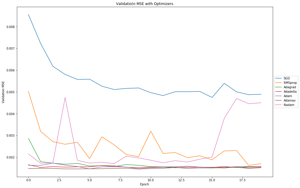
final_model = "Adamax"
model.load_weights("my_model_Adamax.h5")
## TODO: Visualize the training and validation loss of your neural network

# accuracy for training / validation loss
plt.plot(history[final_model].history['acc'])
plt.plot(history[final_model].history['val_acc'])
plt.title('model accuracy for training / validation set')
plt.ylabel('accuracy')
plt.xlabel('epoch')
plt.legend(['train', 'test'], loc='upper left')
plt.show()

# summarize history for loss
plt.plot(history[final_model].history['loss'])
plt.plot(history[final_model].history['val_loss'])
plt.title('traning and validation loss')
plt.ylabel('loss')
plt.xlabel('epoch')
plt.legend(['train', 'test'], loc='upper left')
plt.show()

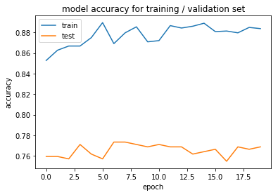

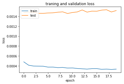
Question 3: Do you notice any evidence of overfitting or underfitting in the above plot? If so, what steps have you taken to improve your model? Note that slight overfitting or underfitting will not hurt your chances of a successful submission, as long as you have attempted some solutions towards improving your model (such as regularization, dropout, increased/decreased number of layers, etc).
Answer:
Execute the code cell below to visualize your model’s predicted keypoints on a subset of the testing images.
y_test = model.predict(X_test)
fig = plt.figure(figsize=(20,20))
fig.subplots_adjust(left=0, right=1, bottom=0, top=1, hspace=0.05, wspace=0.05)
for i in range(9):
    ax = fig.add_subplot(3, 3, i + 1, xticks=[], yticks=[])
    plot_data(X_test[i], y_test[i], ax)

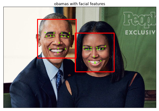
With the work you did in Sections 1 and 2 of this notebook, along with your freshly trained facial keypoint detector, you can now complete the full pipeline. That is given a color image containing a person or persons you can now
In this Subsection you will do just this!
Use the OpenCV face detection functionality you built in previous Sections to expand the functionality of your keypoints detector to color images with arbitrary size. Your function should perform the following steps
Note: step 4 can be the trickiest because remember your convolutional network is only trained to detect facial keypoints in $96 \times 96$ grayscale images where each pixel was normalized to lie in the interval $[0,1]$, and remember that each facial keypoint was normalized during training to the interval $[-1,1]$. This means - practically speaking - to paint detected keypoints onto a test face you need to perform this same pre-processing to your candidate face - that is after detecting it you should resize it to $96 \times 96$ and normalize its values before feeding it into your facial keypoint detector. To be shown correctly on the original image the output keypoints from your detector then need to be shifted and re-normalized from the interval $[-1,1]$ to the width and height of your detected face.
When complete you should be able to produce example images like the one below
<img src=”images/obamas_with_keypoints.png” width=1000 height=1000/>
### TODO: Use the face detection code we saw in Section 1 with your trained conv-net

# Load in color image for face detection
image = cv2.imread('images/obamas4.jpg')

# Convert the image to RGB colorspace
image = cv2.cvtColor(image, cv2.COLOR_BGR2RGB)

gray = cv2.cvtColor(image, cv2.COLOR_RGB2GRAY)

# Extract the pre-trained face detector from an xml file
face_cascade = cv2.CascadeClassifier('detector_architectures/haarcascade_frontalface_default.xml')

# Detect the faces in image
faces = face_cascade.detectMultiScale(gray, 2, 2)

# Print the number of faces detected in the image
print('Number of faces detected:', len(faces))

# Make a copy of the orginal image to draw face detections on
image_copy = np.copy(image)

predicted_points = []
# Get the bounding box for each detected face
for (x,y,w,h) in faces:
    crop_img = gray[y:y+h, x:x+w]
    resized_crop_image = cv2.resize(crop_img, (96, 96))
    reshape_img = np.reshape(resized_crop_image, (96,96,1)) / 255

    predicted_points.append(reshape_img)

    # Add a red bounding box to the detections image
    cv2.rectangle(image_copy, (x,y), (x+w,y+h), (255,0,0), 3)

predicted_points = model.predict(np.array(predicted_points))

# plot our image and the detected facial points
fig = plt.figure(figsize = (9,9))
ax1 = fig.add_subplot(111)
ax1.set_xticks([])
ax1.set_yticks([])

for i in range(predicted_points.shape[0]):
    orig_x,orig_y,orig_w,orig_h = faces[i]

    # denormalize points
    pts_x = predicted_points[i][0::2] * orig_w/2 + orig_w/2 + orig_x
    pts_y = predicted_points[i][1::2] * orig_h/2 + orig_h/2 + orig_y

    ax1.scatter(pts_x,pts_y, marker='o', c='lawngreen', s=10)


ax1.set_title('obamas with facial features')
ax1.imshow(image_copy)
Number of faces detected: 2


<matplotlib.image.AxesImage at 0x7fc42bfcde48>

Now you can add facial keypoint detection to your laptop camera - as illustrated in the gif below.
<img src=”images/facial_keypoint_test.gif” width=400 height=300/>
The next Python cell contains the basic laptop video camera function used in the previous optional video exercises. Combine it with the functionality you developed for keypoint detection and marking in the previous exercise and you should be good to go!
import cv2
import time
from keras.models import load_model
def laptop_camera_go():
    # Create instance of video capturer
    cv2.namedWindow("face detection activated")
    vc = cv2.VideoCapture(0)

    # Try to get the first frame
    if vc.isOpened():
        rval, frame = vc.read()
    else:
        rval = False

    # keep video stream open
    while rval:
        # plot image from camera with detections marked
        cv2.imshow("face detection activated", frame)

        # exit functionality - press any key to exit laptop video
        key = cv2.waitKey(20)
        if key > 0: # exit by pressing any key
            # destroy windows
            cv2.destroyAllWindows()

            # hack from stack overflow for making sure window closes on osx --> https://stackoverflow.com/questions/6116564/destroywindow-does-not-close-window-on-mac-using-python-and-opencv
            for i in range (1,5):
                cv2.waitKey(1)
            return

        # read next frame
        time.sleep(0.05)             # control framerate for computation - default 20 frames per sec
        rval, frame = vc.read()
# Run your keypoint face painter
laptop_camera_go()
Using your freshly minted facial keypoint detector pipeline you can now do things like add fun filters to a person’s face automatically. In this optional exercise you can play around with adding sunglasses automatically to each individual’s face in an image as shown in a demonstration image below.
<img src=”images/obamas_with_shades.png” width=1000 height=1000/>
To produce this effect an image of a pair of sunglasses shown in the Python cell below.
# Load in sunglasses image - note the usage of the special option
# cv2.IMREAD_UNCHANGED, this option is used because the sunglasses
# image has a 4th channel that allows us to control how transparent each pixel in the image is
sunglasses = cv2.imread("images/sunglasses_4.png", cv2.IMREAD_UNCHANGED)

# Plot the image
fig = plt.figure(figsize = (6,6))
ax1 = fig.add_subplot(111)
ax1.set_xticks([])
ax1.set_yticks([])
ax1.imshow(sunglasses)
ax1.axis('off');

This image is placed over each individual’s face using the detected eye points to determine the location of the sunglasses, and eyebrow points to determine the size that the sunglasses should be for each person (one could also use the nose point to determine this).
Notice that this image actually has 4 channels, not just 3.
# Print out the shape of the sunglasses image
print ('The sunglasses image has shape: ' + str(np.shape(sunglasses)))
The sunglasses image has shape: (1123, 3064, 4)
It has the usual red, blue, and green channels any color image has, with the 4th channel representing the transparency level of each pixel in the image. Here’s how the transparency channel works: the lower the value, the more transparent the pixel will become. The lower bound (completely transparent) is zero here, so any pixels set to 0 will not be seen.
This is how we can place this image of sunglasses on someone’s face and still see the area around of their face where the sunglasses lie - because these pixels in the sunglasses image have been made completely transparent.
Lets check out the alpha channel of our sunglasses image in the next Python cell. Note because many of the pixels near the boundary are transparent we’ll need to explicitly print out non-zero values if we want to see them.
# Print out the sunglasses transparency (alpha) channel
alpha_channel = sunglasses[:,:,3]
print ('the alpha channel here looks like')
print (alpha_channel)

# Just to double check that there are indeed non-zero values
# Let's find and print out every value greater than zero
values = np.where(alpha_channel != 0)
print ('\n the non-zero values of the alpha channel look like')
print (values)
the alpha channel here looks like
[[0 0 0 ..., 0 0 0]
 [0 0 0 ..., 0 0 0]
 [0 0 0 ..., 0 0 0]
 ...,
 [0 0 0 ..., 0 0 0]
 [0 0 0 ..., 0 0 0]
 [0 0 0 ..., 0 0 0]]

 the non-zero values of the alpha channel look like
(array([  17,   17,   17, ..., 1109, 1109, 1109]), array([ 687,  688,  689, ..., 2376, 2377, 2378]))
This means that when we place this sunglasses image on top of another image, we can use the transparency channel as a filter to tell us which pixels to overlay on a new image (only the non-transparent ones with values greater than zero).
One last thing: it’s helpful to understand which keypoint belongs to the eyes, mouth, etc. So, in the image below, we also display the index of each facial keypoint directly on the image so that you can tell which keypoints are for the eyes, eyebrows, etc.
<img src=”images/obamas_points_numbered.png” width=500 height=500/>
With this information, you’re well on your way to completing this filtering task! See if you can place the sunglasses automatically on the individuals in the image loaded in / shown in the next Python cell.
# Load in color image for face detection
image = cv2.imread('images/obamas4.jpg')

# Convert the image to RGB colorspace
image = cv2.cvtColor(image, cv2.COLOR_BGR2RGB)


# Plot the image
fig = plt.figure(figsize = (8,8))
ax1 = fig.add_subplot(111)
ax1.set_xticks([])
ax1.set_yticks([])
ax1.set_title('Original Image')
ax1.imshow(image)
<matplotlib.image.AxesImage at 0x7fc42a480908>

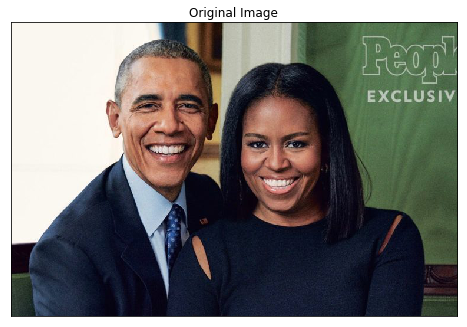
## (Optional) TODO: Use the face detection code we saw in Section 1 with your trained conv-net to put
## sunglasses on the individuals in our test image
## (Optional) TODO: Use the face detection code we saw in Section 1 with your trained conv-net to put
## sunglasses on the individuals in our test image
### TODO: Use the face detection code we saw in Section 1 with your trained conv-net

# Load in color image for face detection
image = cv2.imread('images/obamas4.jpg')

# Convert the image to RGB colorspace
image = cv2.cvtColor(image, cv2.COLOR_BGR2RGB)

gray = cv2.cvtColor(image, cv2.COLOR_RGB2GRAY)

# Extract the pre-trained face detector from an xml file
face_cascade = cv2.CascadeClassifier('detector_architectures/haarcascade_frontalface_default.xml')

# Detect the faces in image
faces = face_cascade.detectMultiScale(gray, 2, 2)

# Print the number of faces detected in the image
print('Number of faces detected:', len(faces))

# Make a copy of the orginal image to draw face detections on
image_copy = np.copy(image)

predicted_points = []
# Get the bounding box for each detected face
for (x,y,w,h) in faces:

    crop_img = gray[y:y+h, x:x+w]
    resized_crop_image = cv2.resize(crop_img, (96, 96))
    reshape_img = np.reshape(resized_crop_image, (96,96,1)) / 255

    predicted_points.append(reshape_img)

    # Add a red bounding box to the detections image
    cv2.rectangle(image_copy, (x,y), (x+w,y+h), (255,0,0), 3)

predicted_points = model.predict(np.array(predicted_points))

# plot our image
fig = plt.figure(figsize = (9,9))
ax1 = fig.add_subplot(111)
ax1.set_xticks([])
ax1.set_yticks([])

for i in range(predicted_points.shape[0]):
    orig_x,orig_y,orig_w,orig_h = faces[i]

    # denormalize points for facial features
    pts_x = predicted_points[i][0::2] * orig_w/2 + orig_w/2 + orig_x
    pts_y = predicted_points[i][1::2] * orig_h/2 + orig_h/2 + orig_y

    sunglasses_height = int((pts_y[10] - pts_y[9])/1.1)
    sunglasses_width = int((pts_x[7] - pts_x[9]) * 1.1)

    sunglasses_top_left_y = int(pts_y[9])
    sunglasses_top_left_x = int(pts_x[9])

    # resized sunglasses
    resized_sunglasses = cv2.resize(sunglasses, (sunglasses_width, sunglasses_height))

    # region that is transparent
    alpha_region = resized_sunglasses[:,:,3] != 0

    image_copy[sunglasses_top_left_y:sunglasses_top_left_y+sunglasses_height, sunglasses_top_left_x:sunglasses_top_left_x+sunglasses_width,:][alpha_region] = resized_sunglasses[:,:,:3][alpha_region]

ax1.set_title('obamas with sunglasses')
ax1.imshow(image_copy)
Number of faces detected: 2


<matplotlib.image.AxesImage at 0x7fc42a468e80>

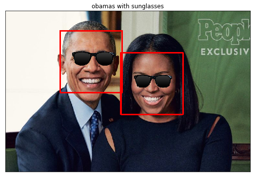
Now you can add the sunglasses filter to your laptop camera - as illustrated in the gif below.
<img src=”images/mr_sunglasses.gif” width=250 height=250/>
The next Python cell contains the basic laptop video camera function used in the previous optional video exercises. Combine it with the functionality you developed for adding sunglasses to someone’s face in the previous optional exercise and you should be good to go!
import cv2
import time
from keras.models import load_model
import numpy as np

def laptop_camera_go():
    # Create instance of video capturer
    cv2.namedWindow("face detection activated")
    vc = cv2.VideoCapture(0)

    # try to get the first frame
    if vc.isOpened():
        rval, frame = vc.read()
    else:
        rval = False

    # Keep video stream open
    while rval:
        # Plot image from camera with detections marked
        cv2.imshow("face detection activated", frame)

        # Exit functionality - press any key to exit laptop video
        key = cv2.waitKey(20)
        if key > 0: # exit by pressing any key
            # Destroy windows
            cv2.destroyAllWindows()

            for i in range (1,5):
                cv2.waitKey(1)
            return

        # Read next frame
        time.sleep(0.05)             # control framerate for computation - default 20 frames per sec
        rval, frame = vc.read()
# Load facial landmark detector model
model = load_model('my_model.h5')

# Run sunglasses painter
laptop_camera_go()